Gradient Descent in Artificial Neural Network

Back to: Data Science Tutorials

Gradient Descent in Artificial Neural Network

In this article, I am going to discuss Gradient Descent in Artificial Neural Networks. Please read our previous article where we discussed How does Artificial Neural Network Work.

Gradient Descent in Artificial Neural Network

It is an optimization algorithm applied to model training. Gradient Descent, to put it simply, identifies the variables that minimize the cost function (error in prediction). Gradient Descent does this by iteratively moving in the opposite direction of the gradient toward a set of parameter values that minimize the function.

The slope of the tangent of the function’s graph, which points in the direction of the greatest rate of rising for the function, is represented by a gradient, which is a vector-valued function. It is a derivative that shows the cost function’s slope or inclines.

Imagine being on top of a mountain. The bottom field is where you want to go, but there’s a problem: you’re blind. What do you think of a solution? You’ll need to circle around and advance in the direction of the steeper hill in modest stages. You repeat this process several times, going down the mountain one step at a time.

Gradient Descent does exactly that. It intends to descend to the mountain’s base. The mountain is represented by the data plotted in space, the learning rate is represented by the size of the step you take, and the gradient of a set of parameter values is calculated repeatedly while you feel the incline around you to determine which is higher. Where the cost function decreases are the preferred direction (the opposite direction of the gradient). The value (or weights) at which the function’s cost fell to its lowest in the mountain’s lowest point (the parameters where our model presents more accuracy).

Let’s understand a very important term for Gradient Descent.

As we previously stated, the gradient is a vector-valued function with a direction and magnitude. To find the following point, the Gradient Descent algorithm multiplies the gradient by a constant (Learning rate or Step size).

The gradient descent process will choose the next point 0.042 distant from the previous point, for instance, if the gradient has a magnitude of 4.2 and a learning rate of 0.01.

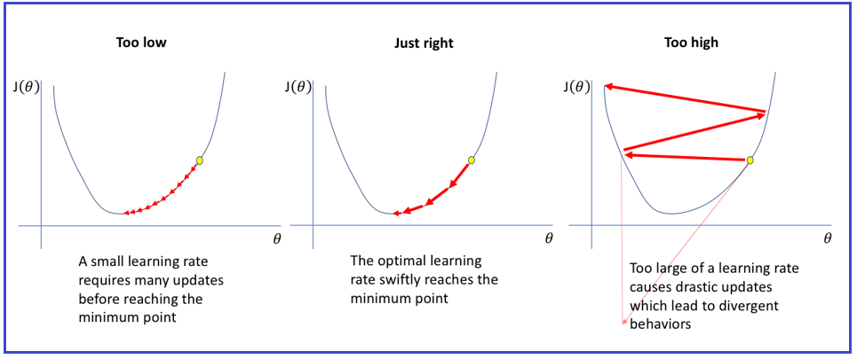
If you experimented with the link’s learning rate, you obviously know the solution. The learning rate’s value is one of the issues. The learning rate, which is determined at random, indicates how far to move the weights. If your learning rate is low, it will take you a long time to reach the minima; if it is high, you will pass the minima.

The learning rate is typically chosen manually, starting with common values of 0.1, 0.01, or 0.001, and then be adjusted if the gradient descent is taking too long to calculate (you need to increase the learning rate), or exploding or behaving erratically (you need to decrease the learning rate).

Gradient Descent Algorithm in Detail-

We’ll refer to the Agent as the blindfolded person in keeping with the mountain scenario. The agent only understands two things for each position: the gradient (for those parameters, or positions) and the breadth of the step to be taken (learning rate). Each parameter’s present value is changed using that knowledge. The gradient is recalculated using the updated parameter values, and the procedure is continued until convergence or local minima are reached.

Let’s go over each stage of the gradient descent technique once more:

Repeat until convergence is reached:

1. Determine the change in the parameters with the learning rate given the gradient.
2. Recalculate the gradient using the new parameter value.
3. Re-do step 1

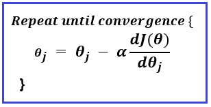
Here is the gradient descent algorithm’s formula:

When the loss function does not considerably improve and we are trapped close to the minima, the scenario is known as convergence.

Gradient Descent Variants

Depending on how much information was utilized to determine the gradient, there are three types of gradient descent:

1. Batch Gradient Descent
2. Stochastic Gradient Descent
3. Mini-batch Gradient Descent

Batch Gradient Descent –

The error for each observation in the dataset is calculated via batch gradient descent, also known as vanilla gradient descent, however, an update is only made after all observations have been reviewed. Because the complete dataset must be kept in memory, batch gradient descent consumes a significant amount of processing resources.

Stochastic Gradient Descent –

For each observation, stochastic gradient descent (SGD) updates a parameter. As a result, it just requires one observation to update the parameter rather than looping through all of them. SGD is typically faster than batch gradient descent, however, because of its frequent updates, the error rate has a bigger variance and occasionally jumps instead of declining.

Mini-Batch Gradient Descent –

It combines stochastic gradient descent with bath gradient descent. A batch of observations receives an update thanks to mini-batch gradient descent. The batch sizes for this approach, which is preferred for neural networks, are typically between 50 and 256.

Stochastic Gradient Descent

Stochastic gradient descent is a well-liked and often used method that is the foundation of Neural Networks and other Machine Learning algorithms.

The gradient descent algorithm has a few drawbacks. We need to pay more attention to how much computation we perform throughout each algorithm iteration.

Let’s say we have 10 characteristics and 10,000 data points. There are as many terms in the sum of squared residuals as there are data points or 10,000 terms in our example. In order to calculate this function’s derivative with respect to each of the characteristics, we must perform 10,000 × 10, or 100,000 computations, per iteration. Since 1000 iterations are typical, the algorithm will require 100,000 * 1000 = 100 000 000 calculations to complete. Gradient descent is slow on large amounts of data because that is essentially an overhead.

Our savior is stochastic gradient descent! Simply said, the word “stochastic” means “random.”

Where in our gradient descent technique can we possibly include randomness?

Yes, it appears that your guess was accurate! At each stage, the derivatives are calculated while choosing data points. In order to drastically reduce calculations, SGD chooses one data point at random from the entire data set for each iteration.

Another typical practice is known as “mini-batch” gradient descent, which involves sampling a small number of data points rather than just one at each step.

Single Perceptron and its Limitations

The most widely used term in machine learning and artificial intelligence is perceptron, which is used by all people. Learning machine learning and deep learning technologies, which are made up of a set of weights, input values or scores, and a threshold is the first step in this process. A component of an artificial neural network is the perceptron.

Single perceptrons are single Artificial Neurons or Neural Network Units that are used in Business Intelligence to help detect certain input data computations. They have four primary parameters: input values, weights and bias, net sum, and activation function.

The single-layer perceptron model’s primary goal is to examine things that can be linearly separated into binary categories.

A single-layer perceptron model starts with randomly assigned input for the weight parameters because its methods do not use recorded data. Additionally, it totals all inputs (weight). The model is active and displays the output result as +1 if, after combining all inputs, the total sum exceeds a certain value.

The performance of this model is said to be satisfied if the result is the same as the predetermined value or threshold value, and the weight demand remains constant. However, this model has a few inconsistencies that arise when different weight input values are used.

In order to identify the intended output and reduce errors, various adjustments to the weights input should be required.

Limitations of Single Perceptron –

1. The hard limit transfer function of a perceptron limits the output to a binary number (0 or 1) alone.
2. Only sets of input vectors that can be linearly separated can be classified using perceptrons. Non-linear input vectors are difficult to correctly categorize.

Multi-Layered Perceptron Model

A multi-layer perceptron model has more hidden layers than a single-layer perceptron model, but both share the same model structure.

The backpropagation algorithm, commonly known as the multi-layer perceptron model, runs in two steps as follows:

1. Forward Stage: In the forward stage, activation operations begin at the input layer and end at the output layer.
2. Backward Stage: Weight and bias variables are adjusted in the backward stage to meet the needs of the model. At this point, the discrepancy between the requested output and the actual output started on the output layer and concluded on the input layer.

As a result, a multi-layered perceptron model has been compared to several artificial neural networks with different layers in which the activation function is not linear, comparable to a single-layer perceptron model. For deployment, activation functions other than linear can be used, such as sigmoid, TanH, ReLU, etc.

Advantages of Multi-Layered Perceptron Model –

1. A multi-layer perceptron model can process both linear and non-linear patterns and has more processing capability.
2. With both little and large input data, it functions well.
3. We can make quick predictions using it after training.
4. It is beneficial to get the same accuracy ratio with both large and little data.

Disadvantages of Multi-Layered Perceptron Model –

1. Computations in the multi-layer perceptron are challenging and time-consuming.
2. It is challenging to estimate how much the dependent variable will influence each independent variable in a multi-layer perceptron.
3. The effectiveness of the model depends on how well it was trained.

In the next article, I am going to discuss Deep Neural Networks. Here, in this article, I try to explain the Gradient Descent in Artificial Neural Networks. I hope you enjoy this Gradient Descent in Artificial Neural Network article. Please post your feedback, suggestions, and questions about this Gradient Descent in Artificial Neural Network article.