Building a Real World Convolutional Neural Network for Image Classification

Back to: Data Science Tutorials

Building a Real World Convolutional Neural Network for Image Classification

All the neurons in RegularNets are connected to one another, which is its fundamental structural trait. For instance, when we have greyscale images that are 28 by 28, we will have 784 (28 x 28 x 1) neurons in a layer that appears manageable. Many photos, nevertheless, have many more pixels and are not in grayscale. With 26,542,080 (4096 x 2160 x 3) unique neurons connected to one another in the first layer, assuming we have a set of color images in 4K Ultra HD, this problem is not solvable. As a result, we can conclude that RegularNets cannot be scaled for picture categorization.

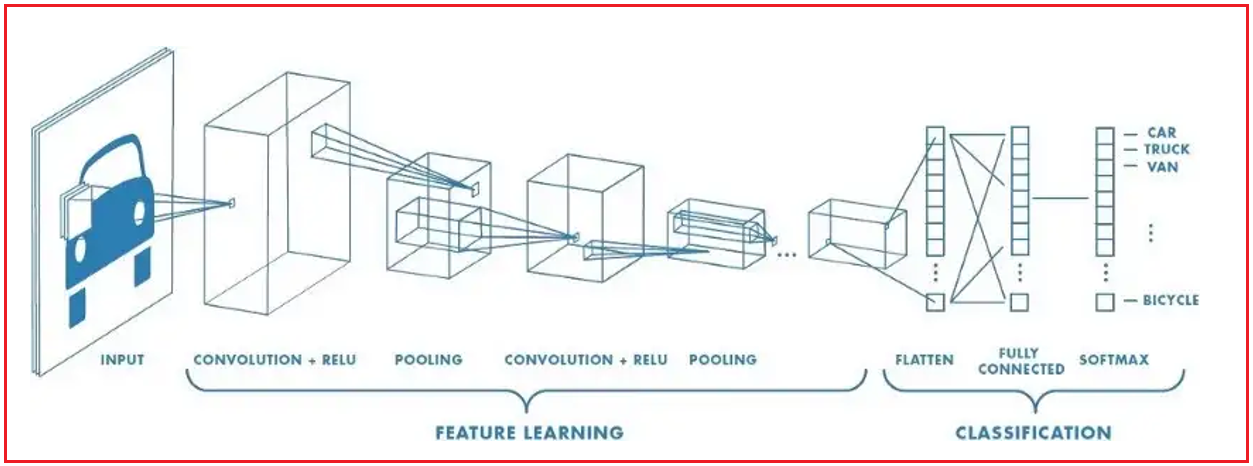
However, it appears that there is little correlation or relationship between two individual pixels until they are close to one another, particularly when it comes to images. Convolutional and pooling layers are the result of this. A convolutional neural network can have a wide variety of layers. The most crucial layers, however, are convolution, pooling, and completely linked.

Our RegularNet is a completely connected network where each parameter is connected to another to establish the true relationship and impact of each parameter on the labels. We can ultimately build a fully connected network to categorize our photos since convolution and pooling layers significantly lower our time-space complexity. The following describes a set of fully connected layers:

One of the most popular datasets for image classification is the MNIST dataset, which is available from a variety of sources. In fact, we can import and download the MNIST dataset straight via Tensorflow and Keras’s APIs. I will start by importing the TensorFlow and MNIST datasets using the following two lines of the Keras API.

The MNIST database includes 60,000 training images and 10,000 test images from American high school students and Census Bureau employees, respectively. Therefore, I have divided these two groups into train and test, as well as the labels and the photos, in the second line. While y train and y test sections have labels from 0 to 9 that indicate what number they truly are, x train and x test portions have greyscale RGB codes (from 0 to 255). We can use matplotlib’s assistance to visualize these numbers.

# Import Libraries and download dataset
import tensorflow as tf
import matplotlib.pyplot as plt
(x_train, y_train), (x_test, y_test) = tf.keras.datasets.mnist.load_data()

# We have total 60,000 train images so we can select any random image index between 0 to 59999
image_index = 9000 
print(y_train[image_index])
plt.imshow(x_train[image_index], cmap='Greys')

In order to feed the dataset to the convolutional neural network, we also need to know its structure.

You’ll receive (60000, 28, 28). 60000 denotes the total number of images in the train dataset, and (28, 28) denotes the image size, which is 28 x 28 pixels. We require 4-dims NumPy arrays in order to use the dataset using the Keras API. But as we can see above, our array is a 3-dim one. Additionally, we must normalize our data because neural network models constantly demand it. To do this, we must divide the RGB codes by 255. (which is the maximum RGB code minus the minimum RGB code).

# Reshaping the array to 4-dimension
x_train = x_train.reshape(x_train.shape[0], 28, 28, 1)
x_test = x_test.reshape(x_test.shape[0], 28, 28, 1)
input_shape = (28, 28, 1)
# converting values to float
x_train = x_train.astype('float32')
x_test = x_test.astype('float32')
# Normalizing the RGB codes
# We can do so by dividing it to the max RGB value (255)
x_train /= 255
x_test /= 255
print('x_train shape:', x_train.shape)
print('Number of images in x_train', x_train.shape[0])
print('Number of images in x_test', x_test.shape[0])

We’ll use Keras, which is the most simple API (which uses either TensorFlow or Theano on the backend). Therefore, I will add Conv2D, MaxPooling, Flatten, Dropout, and Dense layers to the imported Sequential Model from Keras. Max pooling, Dense layers, and Conv2D have already been covered. Additionally, Dropout layers combat overfitting by ignoring a portion of the neurons during training, whereas Flatten layers first create the fully linked layers by flattening 2D arrays to 1D arrays.

# Importing the required Keras modules containing model and layers
from tensorflow.keras.models import Sequential
from tensorflow.keras.layers import Dense, Conv2D, Dropout, Flatten, MaxPooling2D

# Creating a Sequential Model and adding the layers
model = Sequential()
model.add(Conv2D(28, kernel_size=(3,3), input_shape=input_shape))
model.add(MaxPooling2D(pool_size=(2, 2)))

# Flattening the 2D arrays for fully connected layers
model.add(Flatten()) 
model.add(Dense(128, activation=tf.nn.relu))
model.add(Dropout(0.2))
model.add(Dense(10,activation=tf.nn.softmax))

For the first Dense layer, we can experiment with any number; however, because there are 10 different number classes (0, 1, 2,…, 9), the final Dense layer must have 10 neurons. To improve the outcome, you may always play about with the first Dense layer’s kernel size, pool size, activation functions, dropout rate, and the number of neurons. Set an optimizer with a predetermined loss function that makes use of a metric now. Using our train data, we can then fit the model.

model.compile(optimizer='adam', 
              loss='sparse_categorical_crossentropy', 
              metrics=['accuracy'])
model.fit(x=x_train,y=y_train, epochs=10)
model.evaluate(x_test, y_test)

Now, let us check how well the model is able to make classification on test data –

# Let's test how the model is performing on the test set
image_index = 4000
plt.imshow(x_test[image_index].reshape(28, 28),cmap='Greys')
pred = model.predict(x_test[image_index].reshape(1, 28, 28, 1))
print(pred.argmax())

Here, in this article, I try to explain Building a Real World Convolutional Neural Network for Image Classification. I hope you enjoy this Building a Real World Convolutional Neural Network for Image Classification article. Please post your feedback, suggestions, and questions about this article.