Case Study in Image Recognition Domain

Back to: Data Science Tutorials

Case Study in the Image Recognition Domain

In this article, I am going to discuss a Case Study in the Image Recognition Domain. Please read our previous article where we discussed Recurrent Neural Networks (RNNs).

A Case Study in the Image Recognition Domain

Everyone understands a computer understands the language of numbers. So how it processes images? Let us understand what images are made of.

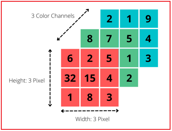
A digital image is one that is made up of picture components, also referred to as pixels, each of which has a definite, finite amount of numeric representation for its level of intensity. Two categories of images exist:

1. Binary Image – As its name implies, a binary image consists of just two-pixel elements, 0 and 1, where 0 denotes black and 1 denotes white.
2. Colored Images – An RGB-formatted colored image is a result of combining data from three separate matrices. It gives a description of the color that each pixel in the image exhibits. To do this, the red component is defined in the first matrix, followed by the green component in the second, and the blue component in the last matrix.

Each pixel on the screen comprises three different color components: red, green, and blue. The RGB value of the pixel is widely used to describe these. Assume, for illustration, that a pixel’s red, green, and blue values (intensities) can each have 256 possible values (0 through 255). An RGB value of (0, 255, 0) would indicate a green pixel, an RGB value of (0, 0, 255) would indicate a blue pixel, and an RGB value of (255, 0, 0) would indicate a red pixel. White is represented by the RGB value of (255, 255, 255), while black is represented by (0, 0, 0). The eye can distinguish between a wide spectrum of colors by varying the RGB value of the three-color components.

We quickly learn that a fully-connected neural network does not scale effectively when used for image processing. Each pixel of an image is input into the network for processing. Therefore, we need to supply 200 * 200 * 3 = 120,000 input neurons for an image of size 200x200x3 (i.e. 200 pixels on 200 pixels with 3 color channels, e.g. red, green, and blue). Then, each matrix is 200 by 200 pixels in size, for a total of 200 * 200 entries. Finally, there are three copies of this matrix—one for each of red, blue, and green. This implies that as we increase the number of neurons in the Hidden Layer, the number of parameters would rise rapidly.

A network with so many parameters will almost certainly experience overfitting. This indicates that the model will make accurate predictions for the training set but will struggle to apply its findings to novel cases.

For these reasons, we are unable to train these images using neural networks using a broad technique. Convolutional neural networks can help in this situation. The Convolutional Neural Network adopts a different strategy and imitates how our eyes help us perceive our surroundings. When we perceive a picture, we instantly break it down into numerous smaller sub-images and examine each one separately. We analyze and interpret the image by putting these smaller images together.

Convolution Operation

One of CNN’s key components is convolution. The mathematical combining of two functions to yield a third function is referred to as convolution. It combines two sets of data.

A feature map is created by performing convolution on the input data in the case of a CNN using a filter or kernel (both names are used interchangeably).

The traditional input for a 2D input would be a picture, where we recalculate each pixel’s value by adding up its neighbors’ weighted sums, Suppose the input image is as follows.

The Kernel or Filter is the current name for this weight’s matrix. We have a kernel with a size of 2X2 in the scenario above. Let us take a sample matrix for the input image and a sample 2X2 filter to understand the convolution operation.

The first pixel’s new value would be determined by applying the 2X2 filter to the first 2X2 area of the image and then taking its weighted sum.

This operation would result in the following –

aw+bx+ey+fz

Then, we move the filter horizontally by one and apply it to the following 2 X 2 region of the input; in this example, the pixels of interest are b, c, f, and g.

Using the same method, we compute the output and obtain:

bw+cx+fy+gz

Then, we again move the horizontal kernel/filter by 1 and calculate the weighted sum:

cw+dx+gy+hz

As a result, the output from the first layer would appear as follows:

In general, we move the kernel as follows:

First, we start with the starting portion of the image, move the filter in the horizontal direction, and cover this row completely. Next, we move the filter in the vertical direction (by some amount relative to the top left portion of the image), again striding it horizontally through the entire row, and continue moving the kernel down by 1 in the vertical direction. We essentially move the kernel from top to bottom and from left to right.

So, the next step will be –

The stride is the number of pixels by which we slide the kernel. Normally, the stride is kept at 1, but we can make it longer. In order to fit the kernel at the image’s edges when it is increased, the image size may need to be increased by a few pixels. Padding is the name given to this rise. The usual practice is to use the odd-dimensional kernel.

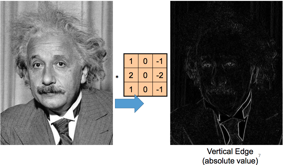
There are a select few filters used in image processing for a variety of tasks. For instance – a filter that can be used to blur photos, sharpen images, conduct edge detection, and do other operations.

CNN’s can extract more meaning from photos than perhaps humans or filters made by humans could by learning the values of various filters.

The filters in a convolutional layer frequently learn to recognize abstract ideas like the edge of a face or a person’s shoulders. Convolutional layer stacking allows us to extract more detailed and abstract information from a CNN. The shape of the eyes, the margins of a shoulder, and other details might be detectable using the second layer of convolution.

Relu Layers

Hidden layers of a trained CNN have neurons that could be abstract representations of the input characteristics. A CNN is not aware of which of the learned abstract representations will apply to a given input when it is presented with an unknown input. There are two possible (fuzzy) scenarios for each neuron in the buried layer that represents a particular learned abstract representation: either the neuron is relevant or it is not.

The absence of one neuron does not necessarily imply the absence of other potential abstract representations as a result. If we used an activation function whose image is, then the output of a neuron would be negatively correlated with the output of the neural network for some input values.

We presume that all learned abstract representations are independent of one another, which is often undesirable. Therefore, non-negative activation functions are preferred for CNNs. The Rectified Linear function is the most prevalent of these functions, and a neuron that employs it is known as a Rectified Linear Unit (ReLU) –

Compared to sigmoidal functions, this function has two key advantages:

1. ReLU can be calculated extremely easy because all that is required is to compare the input to the value 0.
2. Additionally, depending on whether its input is negative, it has a derivative of either 0 or 1.

The latter has significant ramifications for training-related backpropagation. It means that computing the gradient of a neuron is not expensive:

On the other hand, sigmoidal activation functions and other non-linear activation functions typically lack this property. As a result, using ReLU lessens the likelihood that the computing needed to run the neural network would rise exponentially. The computational cost of adding additional ReLUs rises linearly as the CNN’s size scales.

The so-called “vanishing gradient” problem, which frequently occurs when using sigmoidal functions, is likewise avoided by ReLUs. This issue relates to a neuron’s propensity for its gradient to approach zero for large input levels. ReLU always stays at a constant 1, unlike sigmoidal functions, whose derivatives tend to 0 as they approach positive infinity.

In the next article, I am going to discuss SoftMax vs Cross Entropy in CNN. Here, in this article, I try to explain the Case study in the Image Recognition Domain. I hope you enjoy this Case study in the Image Recognition Domain article. Please post your feedback, suggestions, and questions about this Case study in the Image Recognition Domain article.